dplyr - Data Mainpulation Package
Intorduction
Most of the data scientists spend 80% of their time on data preparation for a given project also known as wrangling or cleaning or simply we can say data manipulations, so dplyr is one of the most popular package which can help R users to solve on preparing or manipulating the dataset before going for actual analysis or modeling. some of those operations such as selecting required columns, adding a new column, filtering required observations, or even some of the tasks like sorting or aggregating
dplyr has couple of functions like
select()
filter()
mutate()
arrange()
summarize()
and %>% operator
Install required packages
load the packages
library(dplyr)
library(ggplot2)
loading and examine the dataset
#for illustration purpose take the diamonds dataset from ggplot2 package and attached to this session
data(diamonds)
#examin first 6 observations
head(diamonds)
## # A tibble: 6 x 10
##   carat cut       color clarity depth table price     x     y     z
##   <dbl> <ord>     <ord> <ord>   <dbl> <dbl> <int> <dbl> <dbl> <dbl>
## 1 0.23  Ideal     E     SI2      61.5    55   326  3.95  3.98  2.43
## 2 0.21  Premium   E     SI1      59.8    61   326  3.89  3.84  2.31
## 3 0.23  Good      E     VS1      56.9    65   327  4.05  4.07  2.31
## 4 0.290 Premium   I     VS2      62.4    58   334  4.2   4.23  2.63
## 5 0.31  Good      J     SI2      63.3    58   335  4.34  4.35  2.75
## 6 0.24  Very Good J     VVS2     62.8    57   336  3.94  3.96  2.48
#take help from r documentation
#?diamonds
#examine the data
dim(diamonds)
## [1] 53940    10
str(diamonds)
## Classes 'tbl_df', 'tbl' and 'data.frame':    53940 obs. of  10 variables:
##  $ carat  : num  0.23 0.21 0.23 0.29 0.31 0.24 0.24 0.26 0.22 0.23 ...
##  $ cut    : Ord.factor w/ 5 levels "Fair"<"Good"<..: 5 4 2 4 2 3 3 3 1 3 ...
##  $ color  : Ord.factor w/ 7 levels "D"<"E"<"F"<"G"<..: 2 2 2 6 7 7 6 5 2 5 ...
##  $ clarity: Ord.factor w/ 8 levels "I1"<"SI2"<"SI1"<..: 2 3 5 4 2 6 7 3 4 5 ...
##  $ depth  : num  61.5 59.8 56.9 62.4 63.3 62.8 62.3 61.9 65.1 59.4 ...
##  $ table  : num  55 61 65 58 58 57 57 55 61 61 ...
##  $ price  : int  326 326 327 334 335 336 336 337 337 338 ...
##  $ x      : num  3.95 3.89 4.05 4.2 4.34 3.94 3.95 4.07 3.87 4 ...
##  $ y      : num  3.98 3.84 4.07 4.23 4.35 3.96 3.98 4.11 3.78 4.05 ...
##  $ z      : num  2.43 2.31 2.31 2.63 2.75 2.48 2.47 2.53 2.49 2.39 ...
summary(diamonds)
##      carat               cut        color        clarity
##  Min.   :0.2000   Fair     : 1610   D: 6775   SI1    :13065
##  1st Qu.:0.4000   Good     : 4906   E: 9797   VS2    :12258
##  Median :0.7000   Very Good:12082   F: 9542   SI2    : 9194
##  Mean   :0.7979   Premium  :13791   G:11292   VS1    : 8171
##  3rd Qu.:1.0400   Ideal    :21551   H: 8304   VVS2   : 5066
##  Max.   :5.0100                     I: 5422   VVS1   : 3655
##                                     J: 2808   (Other): 2531
##      depth           table           price             x
##  Min.   :43.00   Min.   :43.00   Min.   :  326   Min.   : 0.000
##  1st Qu.:61.00   1st Qu.:56.00   1st Qu.:  950   1st Qu.: 4.710
##  Median :61.80   Median :57.00   Median : 2401   Median : 5.700
##  Mean   :61.75   Mean   :57.46   Mean   : 3933   Mean   : 5.731
##  3rd Qu.:62.50   3rd Qu.:59.00   3rd Qu.: 5324   3rd Qu.: 6.540
##  Max.   :79.00   Max.   :95.00   Max.   :18823   Max.   :10.740
##
##        y                z
##  Min.   : 0.000   Min.   : 0.000
##  1st Qu.: 4.720   1st Qu.: 2.910
##  Median : 5.710   Median : 3.530
##  Mean   : 5.735   Mean   : 3.539
##  3rd Qu.: 6.540   3rd Qu.: 4.040
##  Max.   :58.900   Max.   :31.800
##
select()
Select perticular interested columns from the dataset
# select only the variables carat, color and price
select(diamonds, carat, color, price)
## # A tibble: 53,940 x 3
## carat color price
## <dbl> <ord> <int>
## 1 0.23 E 326
## 2 0.21 E 326
## 3 0.23 E 327
## 4 0.290 I 334
## 5 0.31 J 335
## 6 0.24 J 336
## 7 0.24 I 336
## 8 0.26 H 337
## 9 0.22 E 337
## 10 0.23 H 338
## # ... with 53,930 more rowsfilter()
filter acts like subsetting the data based on certain conditions
# examine the factors in cut variable
table(diamonds$cut)
##
## Fair Good Very Good Premium Ideal
## 1610 4906 12082 13791 21551# subsetting or filtering the diamonds dataset where cut==”Premium”
filter(diamonds, cut=="Premium")## # A tibble: 13,791 x 10
## carat cut color clarity depth table price x y z
## <dbl> <ord> <ord> <ord> <dbl> <dbl> <int> <dbl> <dbl> <dbl>
## 1 0.21 Premium E SI1 59.8 61 326 3.89 3.84 2.31
## 2 0.290 Premium I VS2 62.4 58 334 4.2 4.23 2.63
## 3 0.22 Premium F SI1 60.4 61 342 3.88 3.84 2.33
## 4 0.2 Premium E SI2 60.2 62 345 3.79 3.75 2.27
## 5 0.32 Premium E I1 60.9 58 345 4.38 4.42 2.68
## 6 0.24 Premium I VS1 62.5 57 355 3.97 3.94 2.47
## 7 0.290 Premium F SI1 62.4 58 403 4.24 4.26 2.65
## 8 0.22 Premium E VS2 61.6 58 404 3.93 3.89 2.41
## 9 0.22 Premium D VS2 59.3 62 404 3.91 3.88 2.31
## 10 0.3 Premium J SI2 59.3 61 405 4.43 4.38 2.61
## # ... with 13,781 more rowsmutate()
Mutate function is generally used to add variables to our dataset
diamondsNew<- mutate(diamonds, pricePerCarat = price/carat)
#examine the new dataset whether new variable is added or not
head(diamondsNew)
## # A tibble: 6 x 11
## carat cut color clarity depth table price x y z
## <dbl> <ord> <ord> <ord> <dbl> <dbl> <int> <dbl> <dbl> <dbl>
## 1 0.23 Ideal E SI2 61.5 55 326 3.95 3.98 2.43
## 2 0.21 Premium E SI1 59.8 61 326 3.89 3.84 2.31
## 3 0.23 Good E VS1 56.9 65 327 4.05 4.07 2.31
## 4 0.290 Premium I VS2 62.4 58 334 4.2 4.23 2.63
## 5 0.31 Good J SI2 63.3 58 335 4.34 4.35 2.75
## 6 0.24 Very Good J VVS2 62.8 57 336 3.94 3.96 2.48
## # ... with 1 more variable: pricePerCarat <dbl>names(diamondsNew)## [1] "carat" "cut" "color" "clarity"
## [5] "depth" "table" "price" "x"
## [9] "y" "z" "pricePerCarat"arrange()
this function is used to sort or ordering the data
# first we will see the first 6 diamonds price in our dataset
head(diamonds$depth)
## [1] 61.5 59.8 56.9 62.4 63.3 62.8# then we can use arrange function on top of this vector of first six observationds of depth variable
head(arrange(diamonds,depth))## # A tibble: 6 x 10
## carat cut color clarity depth table price x y z
## <dbl> <ord> <ord> <ord> <dbl> <dbl> <int> <dbl> <dbl> <dbl>
## 1 1 Fair G SI1 43 59 3634 6.32 6.27 3.97
## 2 1.09 Ideal J VS2 43 54 4778 6.53 6.55 4.12
## 3 1 Fair G VS2 44 53 4032 6.31 6.24 4.12
## 4 1.43 Fair I VS1 50.8 60 6727 7.73 7.25 3.93
## 5 0.3 Fair E VVS2 51 67 945 4.67 4.62 2.37
## 6 0.7 Fair D SI1 52.2 65 1895 6.04 5.99 3.14# the above output is basically shows in ascending order
# you can use desc() function inside arrange to make descending the data
head(arrange(diamonds,desc(depth)))## # A tibble: 6 x 10
## carat cut color clarity depth table price x y z
## <dbl> <ord> <ord> <ord> <dbl> <dbl> <int> <dbl> <dbl> <dbl>
## 1 0.5 Fair E VS2 79 73 2579 5.21 5.18 4.09
## 2 0.5 Fair E VS2 79 73 2579 5.21 5.18 4.09
## 3 1.03 Fair E I1 78.2 54 1262 5.72 5.59 4.42
## 4 0.99 Fair J I1 73.6 60 1789 6.01 5.8 4.35
## 5 0.9 Fair G SI1 72.9 54 2691 5.74 5.67 4.16
## 6 0.96 Fair G SI2 72.2 56 2438 6.01 5.81 4.28summarize()
This function is used to get the summary statistics of the data its very powerfull when we use this function with the combination of groupby
#to get the average of price variable
summarize(diamonds, avgPrice = mean(price, na.rm = TRUE) )
## # A tibble: 1 x 1
## avgPrice
## <dbl>
## 1 3933.#combination of summarize/summarise with group_by
summarise(group_by(diamonds, cut), mean=mean(price, na.rm = TRUE))## # A tibble: 5 x 2
## cut mean
## <ord> <dbl>
## 1 Fair 4359.
## 2 Good 3929.
## 3 Very Good 3982.
## 4 Premium 4584.
## 5 Ideal 3458.summarize(group_by(diamonds, cut), mean=mean(price, na.rm = TRUE))## # A tibble: 5 x 2
## cut mean
## <ord> <dbl>
## 1 Fair 4359.
## 2 Good 3929.
## 3 Very Good 3982.
## 4 Premium 4584.
## 5 Ideal 3458.%>% operator
The actual power of dplyr package lies in the usage of pipe operator (%>%), its very usefull when ever we required a chain of operations(series of activities) to work on one after another or using one command’s result as input for another command
#Now we will use those above functions filter select and mutate and combine them into one and get the result by using %>% operator
# filter(diamonds, cut=="Premium")
#select(diamonds, carat, color, price)
# diamondsNew<- mutate(diamonds, pricePerCarat = price/carat)


diamondsPipe <- diamonds %>% filter(cut=="Premium") %>% select(carat, color, price) %>% mutate(pricePerCarat = price/carat)
head(diamondsPipe)
## # A tibble: 6 x 4
## carat color price pricePerCarat
## <dbl> <ord> <int> <dbl>
## 1 0.21 E 326 1552.
## 2 0.290 I 334 1152.
## 3 0.22 F 342 1555.
## 4 0.2 E 345 1725
## 5 0.32 E 345 1078.
## 6 0.24 I 355 1479.ggplot2 - Data Visualization Package
R is one of the most powerfull language for visualizations with minimal lines of code ggplot2 is one of the package which can help the analysts to visualising the data by simple plotting to advanced visualisations
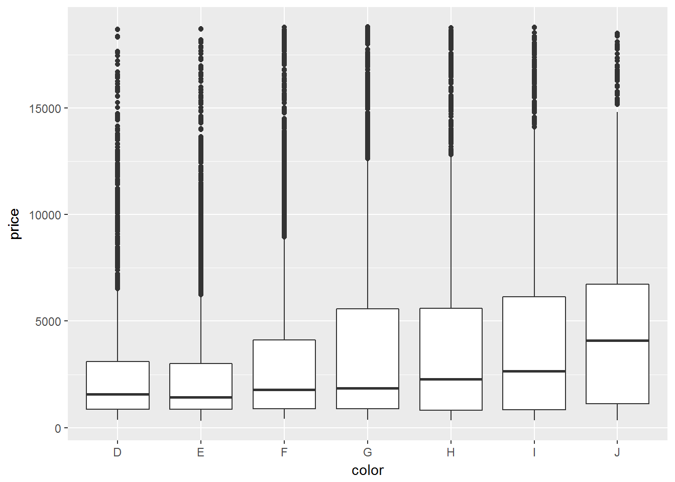
diamonds %>%
  filter(cut == "Ideal") %>%
  ggplot(aes(x=color,y=price)) +
geom_boxplot()